Table of Contents
- 1 1. Create student grades DataFrame object
- 1.1 a. Create a column named
passing_englishthat indicates whether each student has a passing grade in english. - 1.2 b. Sort the english grades by the
passing_englishcolumn. How are duplicates handled? - 1.3 c. Sort the english grades first by
passing_englishand then by studentname. - 1.4 d. Sort the english grades first by
passing_english, and then by the actualenglishgrade, similar to how we did in the last step. - 1.5 e. Calculate each student's overall grade and add it as a column on the DataFrame. The overall grade is the average of the math, english, and reading grades.
- 1.1 a. Create a column named
- 2 2. Load the mpg dataset. Read the documentation for the dataset and use it for the following questions:
- 2.1 a. How many rows and columns are there?
- 2.2 b. What are the data types of each column?
- 2.3 c. Summarize the dataframe with the
.info()and.describe()methods. - 2.4 d. Rename the
ctycolumn tocityandhwytohighwayusing.rename()method. - 2.5 Another way to rename columns...
- 2.6 e. Do any cars have better city mileage than highway mileage?
- 2.7 f. Create a column named
mileage_difference; this column should contain the difference between highway and city mileage for each car. - 2.8 g. Which car (or cars) has the highest mileage difference?
- 2.9 h. Which compact class car has the lowest highway mileage?
- 2.10 j. Create a column named
average_mileagethat is the mean of the city and highway mileage. - 2.11 k. Which Dodge car has the best average mileage? The worst?
- 3 3. Load the Mammals dataset. Read the documentation for it, and use the data to answer these questions:
- 3.1 a. How many rows and columns are there?
- 3.2 b. What are the data types?
- 3.3 c. Summarize the dataframe with .info and .describe
- 3.4 d. What is the the weight of the fastest animal?
- 3.5 e. What is the overall percentage of specials?
- 3.6 f. How many animals are hoppers that are above the median speed? What percentage is this?
Pandas DataFrames Exercises
Big Idea
The Cycle of Improvement - James Clear (Atomic Habits)
Awareness - identify what you need to improve.
Deliberate practice - focus your conscious effort on the specific area you want to improve.
Habit - with practice, the effortful becomes automatic.
Repeat - begin again.
Objectives
By the end of the lesson and exercises, you will be able to...
- create subsets of data from a pandas DataFrame.
.loc[row_indexer, col_indexer]
.iloc[row_indexer, col_indexer]
df[bool_series]
- create and manipulate columns in a pandas DataFrame.
.drop(columns=)
.rename(columns={'original_name': 'new_name')
.assign(new_column = some_expression_or_calculation)
- sort the data in a pandas DataFrame.
.sort_values(by=column(s))
.sort_index(ascending=True)
- chain methods to perform more complicated data manipulations.
df.drop().rename()
import pandas as pd
import numpy as np

import matplotlib.pyplot as plt
%matplotlib inline

from pydataset import data
1. Create student grades DataFrame object
np.random.seed(123)

students = ['Sally', 'Jane', 'Suzie', 'Billy', 'Ada', 'John', 'Thomas',
            'Marie', 'Albert', 'Richard', 'Isaac', 'Alan']

# randomly generate scores for each student for each subject
# note that all the values need to have the same length here

math_grades = np.random.randint(low=60, high=100, size=len(students))
english_grades = np.random.randint(low=60, high=100, size=len(students))
reading_grades = np.random.randint(low=60, high=100, size=len(students))

df = pd.DataFrame({'name': students,
                   'math': math_grades,
                   'english': english_grades,
                   'reading': reading_grades})
Peek at DataFrame
df.head()
# Use shape attribute

df.shape
# Use info method to view both datatypes and potential missing values

df.info()
# Use the `.describe()` method to produce descriptive statistics for columns with numeric datatypes

df.describe()
a. Create a column named passing_english that indicates whether each student has a passing grade in english.
# Create a boolean Series or a boolean mask that returns `True` for a passing English grade.

df.english >= 70
# Create a new column in our DataFrame and assign our boolean Series to it.

df['passing_english'] = df.english >= 70
# Check dataframe for new column.

df.head()
# How many people are passing English? Use the `.sum()` function to add the True bool (1) values.

df['passing_english'].sum()
# How many students are failing English? Use the `.sum()` function to add True values for failing.

df['passing_english'] == False
(df['passing_english'] == False).sum()
b. Sort the english grades by the passing_english column. How are duplicates handled?
.sort_valuesreturns a sorted copy of a given DataFrame unlessinplace=True.It looks like duplicate values are handled according to the index value, small to large or ascending.
# DataFrame.sort_values(by, axis=0, ascending=True, inplace=False, kind='quicksort', na_position='last')
# sorts all of the rows in the DF using the column passed

df.sort_values(by='passing_english')
c. Sort the english grades first by passing_english and then by student name.
All the students that are failing english should be first, and within the students who are failing english, they are ordered alphabetically. The same will be true for the students passing english.
# Now we see that Alan comes before Albert because there is a secondary sort going on alphabetically by name

df.sort_values(by=['passing_english', 'name'])
# What if I want the students passing English first but names in alpha order?

df.sort_values(by=['passing_english', 'name'], ascending=[False, True])
d. Sort the english grades first by passing_english, and then by the actual english grade, similar to how we did in the last step.
df.sort_values(by=['passing_english', 'english'])
# Reverse my sort on both columns

df.sort_values(by=['passing_english', 'english'], ascending=[False, False])
e. Calculate each student's overall grade and add it as a column on the DataFrame. The overall grade is the average of the math, english, and reading grades.
The .iloc attribute allows me to access a group of rows and columns by their integer location or position. Notice below that the observations returned match the integer index location passed to .iloc, and the indexing is NOT inclusive. (from Series Review Notebook)
df.iloc[row_indexer, column_indexer]
I could also solve this using .loc if I wanted to use column labels instead of index position.
df.loc[:, 'math': 'reading']
# Here, I'm selecting all rows and columns at index positions 1, 2, 3. Now I can just sum them.

df.iloc[:, 1:4]
# Since I want the total of the columns in each row, I set axis=1 for columns.

df.iloc[:, 1:4].sum(axis=1)
# Assign to variable and use the Series to create the calculated column I want on my df.

totals = df.iloc[:, 1:4].sum(axis=1)
# assign Series back to DataFrame as overall_grade

df['overall_average'] = round((totals / 3), 0).astype(int)
df.head()
2. Load the mpg dataset. Read the documentation for the dataset and use it for the following questions:
data('mpg', show_doc=True)
mpg = data('mpg')
mpg.head()
a. How many rows and columns are there?
mpg.shape
print(f'There are {mpg.shape[0]} rows and {mpg.shape[1]} columns in the mpg DataFrame.')
b. What are the data types of each column?
mpg.dtypes
c. Summarize the dataframe with the .info() and .describe() methods.
.info()shows us that all of the columns have the same number of non-null values..describe()provides us with the descriptive statistics for all columns with numeric dtypes.
mpg.info()
mpg.describe()
d. Rename the cty column to city and hwy to highway using .rename() method.
.rename()takes in a dictionary with the key as the original name and the value as the new name.If you want to change your original DataFrame to reflect your new column names,
inplace=True
mpg.rename(columns={'cty': 'city', 'hwy': 'highway'}, inplace=True)
mpg.head(1)
Another way to rename columns...
This is another way you can rename columns, especially if you want to change many at once.
I can use the
.columnsattribute to grab my column labels; I can go a step further and print out a list of the current columns in the DataFrame by adding the.to_list()method. It's not necessary if I'm just grabbing the column names, but I love getting the nice list.Then, I make any changes I want to the names in the list and reassign them to
df.columns.
mpg = data('mpg')
mpg.head()
mpg.columns.to_list()
mpg.columns = ['manufacturer', 'model', 'displ', 'year', 'cyl', 'trans', 'drv', 'city',
       'highway', 'fl', 'class']
mpg.head(1)
e. Do any cars have better city mileage than highway mileage?
# Create a boolean Series or a boolean Mask

bool_series = mpg.city > mpg.highway
bool_series.head()
# Return a subset of the original DataFrame using the indexing operator.

mpg[bool_series]
# I can do a quick check to validate my findings above. There are no observations that meet this condition.

bool_series.sum()
f. Create a column named mileage_difference; this column should contain the difference between highway and city mileage for each car.
You saw above how to create a new column in a df using bracket notation; this time I'll show you how to create a new column in a df using the
.assign()method.They are both valid ways to create a new column; if you want to create more than one column at once,
.assign()is worth looking into. Choose your flavor...
# This operation returns a Series of differences in mileage for each row. Looks good.

mpg.highway - mpg.city
# This is how I can create a new column in my df from a calculation on two existing columns.
# I can reassign to my original df at this point, or I might want to assign to a new df name.

mpg = mpg.assign(mileage_difference = mpg.highway - mpg.city)
mpg.head()
g. Which car (or cars) has the highest mileage difference?
# Use the `.max()` function to find the max value in the column.

mpg.mileage_difference.max()
# Create a boolean Series where `True` values identify a match with the max mileage_difference.

bool_series = mpg.mileage_difference == mpg.mileage_difference.max()
bool_series.head()
# Pass my bool_series as a selector for rows in my mpg Series.

mpg[bool_series]
# I can get more specific if I like...

mpg[bool_series][['manufacturer', 'model']]
h. Which compact class car has the lowest highway mileage?
# Why doesn't this work??? This is an example of a situation where you have to use bracket notation

mpg.class
# I check and see that I have a column named `class`. What's up?
# 'class' is a reserved word, so I have to use bracket notation to access the column!

mpg.columns
# I'm taking a look at all of the possible values in the column here.

mpg['class'].value_counts()
# Create the bool Series or selector for the compact class of cars.

bool_series = mpg['class'] == 'compact'
bool_series.head()
# Pass my selector to my original DataFrame to get a subset of compact cars.

compacts = mpg[bool_series]
compacts.head()
# Sort the DataFrame by highway mileage

compacts.sort_values(by='highway').head()
# If you want to isolate the compact car with the lowest highway mileage

compacts.sort_values(by='highway').head(1)
The best highway mileage?
# Isolate the compact car with the best highway mileage.

compacts.sort_values(by='highway', ascending=False).head()
# isolate the row using .head() method

compacts.sort_values(by='highway', ascending=False).head(1)
j. Create a column named average_mileage that is the mean of the city and highway mileage.
# Create the calculated column

(mpg.city + mpg.highway) / 2
# Assign the Series back to the original DataFrame as a new column.

mpg['average_mileage'] = (mpg.city + mpg.highway) / 2
mpg.head(2)
k. Which Dodge car has the best average mileage? The worst?
# Create the boolean Series to filter for Dodge vehicles.

bool_series = mpg.manufacturer == 'dodge'
bool_series.head()
# Use the selector to create a subset of only Dodge vehicles.

dodges = mpg[bool_series]
dodges.head()
# Isolate the Dodge with the best average mileage.

dodges.sort_values(by='average_mileage').tail(1)
# Isolate the Dodge with the worst average mileage.

dodges.sort_values(by='average_mileage').head(4)
# another way...

worst_mileage = dodges.average_mileage.min()
worst_mileage
# Compare the average_mileage of each observation to the scalar value of worst_mileage; return ALL values that match.

dodges[dodges.average_mileage == worst_mileage]
3. Load the Mammals dataset. Read the documentation for it, and use the data to answer these questions:
data('Mammals', show_doc=True)
# Load DataFrame and save as `mammals`.

mammals = data('Mammals')
mammals.head()
a. How many rows and columns are there?
mammals.shape
b. What are the data types?
mammals.dtypes
c. Summarize the dataframe with .info and .describe
mammals.info()
mammals.describe()
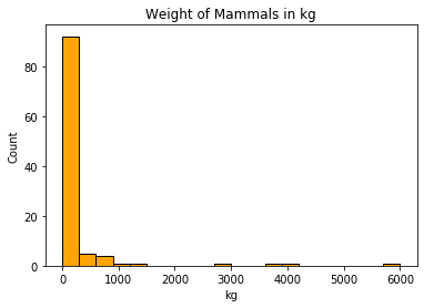
Quick visualization of the distributioin of weight and speed values
plt.hist(mammals.weight, bins=20, color='orange', edgecolor='black')

plt.title('Weight of Mammals in kg')
plt.xlabel('kg')
plt.ylabel('Count')

plt.show()
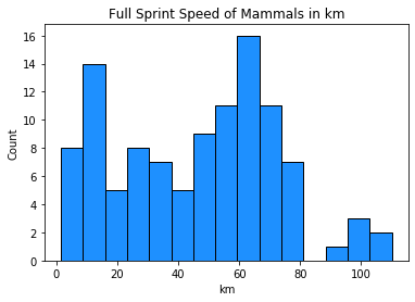
plt.hist(mammals.speed, bins=15, color='dodgerblue', edgecolor='black')

plt.title('Full Sprint Speed of Mammals in km')
plt.xlabel('km')
plt.ylabel('Count')

plt.show()
d. What is the the weight of the fastest animal?
# Find the fastest speed using max(). I see there is only one observation with 110 km.

mammals.speed.value_counts().sort_index(ascending=False).head()
# This returns the index LABEL, not the integer position, and that's why I'm using .loc below. `df.loc[row_label]`

mammals.speed.idxmax()
# I can isolate that observation/mammal using the `.loc` indexer and `.idxmax()` method.

mammals.loc[mammals.speed.idxmax()]
# You guessed it; it's a Series! I can access any of those index labels or values.

type(mammals.loc[mammals.speed.idxmax()])
mammals.loc[mammals.speed.idxmax()].weight
# OR -> I can create a boolan Series to filter for observations that match the max speed.

bool_series = mammals.speed == mammals.speed.max()
bool_series.head()
# Pass my boolean Series to the indexing operator as a selector to find observations that match the fastest speed

mammals[bool_series]
# Isolate the weight value if you want like this...

mammals[bool_series].weight
# or like this without the index label. Again, your context will dictate the data you want to return and how you get it.

mammals.loc[mammals.speed.idxmax()].weight
e. What is the overall percentage of specials?
# We have a boolean Series already.

mammals.specials.head()
# First, I'll find the number of mammals classified as specials.
# True boolean values are understood as having a value of 1, so I can sum the boolean Series.

total_specials = mammals.specials.sum()
total_specials
# Find the total number of mammals in my df.

total_mammals = len(mammals)
total_mammals
print(f'{round(total_specials / total_mammals * 100, 2)}% of mammals in the df are specials.')
f. How many animals are hoppers that are above the median speed? What percentage is this?
- I interpreted this question as animals that are hoppers AND above the median speed for all mammals in our DataFrame.
# Remind myself of column names and values.

mammals.head(1)
# Find the median speed of mammals in our df.

median_speed = mammals.speed.median()
median_speed
# Create boolean Series for mammals with speed above `median_speed` and True for hoppers

bool_series = (mammals.speed > median_speed) & (mammals.hoppers == True)
bool_series.head()
# These are our fast hoppers.

fast_hoppers = mammals[bool_series]
fast_hoppers
len(fast_hoppers)
print(f'This puts fast hoppers at {round((len(fast_hoppers) / len(mammals)) * 100, 2)}% of the mammals.')