Acquire Data for Classification


Big Ideas

  • Cache your data to speed up your data acquisition.

  • Helper functions are your friends.

Objectives

By the end of the acquire lesson and exercises, you will be able to...

  • read data into a pandas DataFrame using the following modules:

pydataset

from pydataset import data
df = data('dataset_name')

seaborn datasets

import seaborn as sns
df = sns.load_dataset('dataset_name')
  • read data into a pandas DataFrame from the following sources:

    • an Excel spreadsheet

    • a Google sheet

    • Codeup's mySQL database

pd.read_excel('file_name.xlsx', sheet_name='sheet_name')
pd.read_csv('filename.csv')
pd.read_sql(sql_query, connection_url)
  • use pandas methods and attributes to do some initial summarization and exploration of your data.
.head()
.shape
.info()
.columns
.dtypes
.describe()
.value_counts()
  • create functions that acquire data from Codeup's database, save the data locally to CSV files (cache your data), and check for CSV files upon subsequent use.

  • create a new python module, acquire.py, that holds your functions that acquire the titanic and iris data and can be imported and called in other notebooks and scripts.


In [1]:
import pandas as pd
import numpy as np

from pydataset import data
import os

import matplotlib.pyplot as plt
import seaborn as sns


# ignore warnings
import warnings
warnings.filterwarnings("ignore")

from env import host, user, password

Create a pandas dataframe, df_iris, from this data.

  • Use a python module (pydata or seaborn datasets) containing datasets as a source for the iris data.

Other Seaborn Datasets you can use are linked here

In [2]:
data('iris', show_doc=True)
iris

PyDataset Documentation (adopted from R Documentation. The displayed examples are in R)

## Edgar Anderson's Iris Data

### Description

This famous (Fisher's or Anderson's) iris data set gives the measurements in
centimeters of the variables sepal length and width and petal length and
width, respectively, for 50 flowers from each of 3 species of iris. The
species are _Iris setosa_, _versicolor_, and _virginica_.

### Usage

    iris
    iris3

### Format

`iris` is a data frame with 150 cases (rows) and 5 variables (columns) named
`Sepal.Length`, `Sepal.Width`, `Petal.Length`, `Petal.Width`, and `Species`.

`iris3` gives the same data arranged as a 3-dimensional array of size 50 by 4
by 3, as represented by S-PLUS. The first dimension gives the case number
within the species subsample, the second the measurements with names `Sepal
L.`, `Sepal W.`, `Petal L.`, and `Petal W.`, and the third the species.

### Source

Fisher, R. A. (1936) The use of multiple measurements in taxonomic problems.
_Annals of Eugenics_, **7**, Part II, 179–188.

The data were collected by Anderson, Edgar (1935). The irises of the Gaspe
Peninsula, _Bulletin of the American Iris Society_, **59**, 2–5.

### References

Becker, R. A., Chambers, J. M. and Wilks, A. R. (1988) _The New S Language_.
Wadsworth & Brooks/Cole. (has `iris3` as `iris`.)

### See Also

`matplot` some examples of which use `iris`.

### Examples

    dni3 <- dimnames(iris3)
    ii <- data.frame(matrix(aperm(iris3, c(1,3,2)), ncol = 4,
                            dimnames = list(NULL, sub(" L.",".Length",
                                            sub(" W.",".Width", dni3[[2]])))),
        Species = gl(3, 50, labels = sub("S", "s", sub("V", "v", dni3[[3]]))))
    all.equal(ii, iris) # TRUE


In [3]:
df_iris = data('iris')

In [4]:
df_iris.head(3)
Out[4]:
Sepal.Length Sepal.Width Petal.Length Petal.Width Species
1 5.1 3.5 1.4 0.2 setosa
2 4.9 3.0 1.4 0.2 setosa
3 4.7 3.2 1.3 0.2 setosa

In [5]:
df_iris.shape
Out[5]:
(150, 5)

In [6]:
df_iris.columns
Out[6]:
Index(['Sepal.Length', 'Sepal.Width', 'Petal.Length', 'Petal.Width',
       'Species'],
      dtype='object')
In [7]:
# Return a nice list of columns if I want to grab and use them later.

df_iris.columns.to_list()
Out[7]:
['Sepal.Length', 'Sepal.Width', 'Petal.Length', 'Petal.Width', 'Species']

In [8]:
# Return just data types.

df_iris.dtypes
Out[8]:
Sepal.Length    float64
Sepal.Width     float64
Petal.Length    float64
Petal.Width     float64
Species          object
dtype: object
In [9]:
# Return data types plus.

df_iris.info()
<class 'pandas.core.frame.DataFrame'>
Int64Index: 150 entries, 1 to 150
Data columns (total 5 columns):
 #   Column        Non-Null Count  Dtype  
---  ------        --------------  -----  
 0   Sepal.Length  150 non-null    float64
 1   Sepal.Width   150 non-null    float64
 2   Petal.Length  150 non-null    float64
 3   Petal.Width   150 non-null    float64
 4   Species       150 non-null    object 
dtypes: float64(4), object(1)
memory usage: 7.0+ KB

  • Would you recommend rescaling the data based on these statistics?

All of the numeric variables in the iris dataset are in the same unit of measure, cm, so I don't see a need to scale them.

IF there were a very large range in our feature values, even though they were measured in the same units, it might be beneficial to scale our data since a number of machine learning algorithms use a distance metric to weight feature importance.

In [10]:
stats = df_iris.describe().T
stats
Out[10]:
count mean std min 25% 50% 75% max
Sepal.Length 150.0 5.843333 0.828066 4.3 5.1 5.80 6.4 7.9
Sepal.Width 150.0 3.057333 0.435866 2.0 2.8 3.00 3.3 4.4
Petal.Length 150.0 3.758000 1.765298 1.0 1.6 4.35 5.1 6.9
Petal.Width 150.0 1.199333 0.762238 0.1 0.3 1.30 1.8 2.5

In [11]:
stats['range'] = stats['max'] - stats['min']
stats[['mean', '50%', 'std', 'range']]
Out[11]:
mean 50% std range
Sepal.Length 5.843333 5.80 0.828066 3.6
Sepal.Width 3.057333 3.00 0.435866 2.4
Petal.Length 3.758000 4.35 1.765298 5.9
Petal.Width 1.199333 1.30 0.762238 2.4
In [12]:
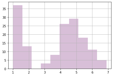
# I can do a quick visual of the variable distributions if I want.

df_iris['Petal.Length'].hist(color='thistle')

plt.show()

Read Table1_CustDetails the excel module dataset, Excel_Exercises.xlsx, into a dataframe, df_excel.

In [13]:
df_excel = pd.read_excel('Spreadsheets_Exercises.xlsx', sheet_name='Table1_CustDetails')
In [14]:
df_excel.info()
<class 'pandas.core.frame.DataFrame'>
RangeIndex: 7049 entries, 0 to 7048
Data columns (total 12 columns):
 #   Column             Non-Null Count  Dtype  
---  ------             --------------  -----  
 0   customer_id        7049 non-null   object 
 1   gender             7049 non-null   object 
 2   is_senior_citizen  7049 non-null   int64  
 3   partner            7049 non-null   object 
 4   dependents         7049 non-null   object 
 5   phone_service      7049 non-null   int64  
 6   internet_service   7049 non-null   int64  
 7   contract_type      7049 non-null   int64  
 8   payment_type       7049 non-null   object 
 9   monthly_charges    7049 non-null   float64
 10  total_charges      7038 non-null   float64
 11  churn              7049 non-null   object 
dtypes: float64(2), int64(4), object(6)
memory usage: 661.0+ KB

I'm going to take care of these categorical variables with numeric data types right now. This will make the rest easier.

In [15]:
df_excel = df_excel.astype({"is_senior_citizen": "object", "phone_service": "object", 
         "internet_service": "object", "contract_type": "object"})

df_excel.info()
<class 'pandas.core.frame.DataFrame'>
RangeIndex: 7049 entries, 0 to 7048
Data columns (total 12 columns):
 #   Column             Non-Null Count  Dtype  
---  ------             --------------  -----  
 0   customer_id        7049 non-null   object 
 1   gender             7049 non-null   object 
 2   is_senior_citizen  7049 non-null   object 
 3   partner            7049 non-null   object 
 4   dependents         7049 non-null   object 
 5   phone_service      7049 non-null   object 
 6   internet_service   7049 non-null   object 
 7   contract_type      7049 non-null   object 
 8   payment_type       7049 non-null   object 
 9   monthly_charges    7049 non-null   float64
 10  total_charges      7038 non-null   float64
 11  churn              7049 non-null   object 
dtypes: float64(2), object(10)
memory usage: 661.0+ KB

Assign the first 100 rows to a new dataframe, df_excel_sample.

In [16]:
df_excel_sample = df_excel.head(100)
In [17]:
df_excel_sample.shape
Out[17]:
(100, 12)

In [18]:
df_excel.shape[0]
Out[18]:
7049

In [19]:
df_excel.columns[:5]
Out[19]:
Index(['customer_id', 'gender', 'is_senior_citizen', 'partner', 'dependents'], dtype='object')

In [20]:
df_excel.select_dtypes(include='object').head()
Out[20]:
customer_id gender is_senior_citizen partner dependents phone_service internet_service contract_type payment_type churn
0 0002-ORFBO Female 0 Yes Yes 1 1 1 Mailed check No
1 0003-MKNFE Male 0 No No 2 1 0 Mailed check No
2 0004-TLHLJ Male 0 No No 1 2 0 Electronic check Yes
3 0011-IGKFF Male 1 Yes No 1 2 0 Electronic check Yes
4 0013-EXCHZ Female 1 Yes No 1 2 0 Mailed check Yes
In [21]:
df_excel.select_dtypes(include='object').columns
Out[21]:
Index(['customer_id', 'gender', 'is_senior_citizen', 'partner', 'dependents',
       'phone_service', 'internet_service', 'contract_type', 'payment_type',
       'churn'],
      dtype='object')

Compute the range for each of the numeric variables.

  • I can choose to look just at the numeric variables quickly like this. If I was going forward with this DataFrame, I would change the data types of numeric categoricals to object data types. I'll wait and do this below with the DataFrames I will use going forward.
In [22]:
telco_stats = df_excel.describe().T
telco_stats
Out[22]:
count mean std min 25% 50% 75% max
monthly_charges 7049.0 64.747014 30.099460 18.25 35.4500 70.35 89.850 118.75
total_charges 7038.0 2283.043883 2266.521984 18.80 401.5875 1397.10 3793.775 8684.80
In [23]:
telco_stats['range'] = telco_stats['max'] - telco_stats['min']
telco_stats
Out[23]:
count mean std min 25% 50% 75% max range
monthly_charges 7049.0 64.747014 30.099460 18.25 35.4500 70.35 89.850 118.75 100.5
total_charges 7038.0 2283.043883 2266.521984 18.80 401.5875 1397.10 3793.775 8684.80 8666.0

Read the data from a Google sheet into a dataframe, df_google.

use this google sheet

In [24]:
# Grab the Google sheet url.

sheet_url = 'https://docs.google.com/spreadsheets/d/1Uhtml8KY19LILuZsrDtlsHHDC9wuDGUSe8LTEwvdI5g/edit#gid=341089357'
In [26]:
# Turn Google sheet address into a CSV export URL.

csv_export_url = sheet_url.replace('/edit#gid=', '/export?format=csv&gid=')
In [27]:
# Read in the data using the pandas `pd.read_csv()` function.

df_google = pd.read_csv(csv_export_url)
In [28]:
df_google.head(3)
Out[28]:
PassengerId Survived Pclass Name Sex Age SibSp Parch Ticket Fare Cabin Embarked
0 1 0 3 Braund, Mr. Owen Harris male 22.0 1 0 A/5 21171 7.2500 NaN S
1 2 1 1 Cumings, Mrs. John Bradley (Florence Briggs Thayer) female 38.0 1 0 PC 17599 71.2833 C85 C
2 3 1 3 Heikkinen, Miss. Laina female 26.0 0 0 STON/O2. 3101282 7.9250 NaN S

In [29]:
df_google.shape
Out[29]:
(891, 12)

In [30]:
df_google.columns.to_list()
Out[30]:
['PassengerId',
 'Survived',
 'Pclass',
 'Name',
 'Sex',
 'Age',
 'SibSp',
 'Parch',
 'Ticket',
 'Fare',
 'Cabin',
 'Embarked']

  • Again, there are numeric data types here that are really categorical variables, so I'll take care of them right here.
In [31]:
df_google.dtypes
Out[31]:
PassengerId      int64
Survived         int64
Pclass           int64
Name            object
Sex             object
Age            float64
SibSp            int64
Parch            int64
Ticket          object
Fare           float64
Cabin           object
Embarked        object
dtype: object
In [32]:
df_google.info()
<class 'pandas.core.frame.DataFrame'>
RangeIndex: 891 entries, 0 to 890
Data columns (total 12 columns):
 #   Column       Non-Null Count  Dtype  
---  ------       --------------  -----  
 0   PassengerId  891 non-null    int64  
 1   Survived     891 non-null    int64  
 2   Pclass       891 non-null    int64  
 3   Name         891 non-null    object 
 4   Sex          891 non-null    object 
 5   Age          714 non-null    float64
 6   SibSp        891 non-null    int64  
 7   Parch        891 non-null    int64  
 8   Ticket       891 non-null    object 
 9   Fare         891 non-null    float64
 10  Cabin        204 non-null    object 
 11  Embarked     889 non-null    object 
dtypes: float64(2), int64(5), object(5)
memory usage: 83.7+ KB
In [33]:
df_google = df_google.astype({'PassengerId': 'object', 'Survived': 'object', 'Pclass': 'object'})
df_google.info()
<class 'pandas.core.frame.DataFrame'>
RangeIndex: 891 entries, 0 to 890
Data columns (total 12 columns):
 #   Column       Non-Null Count  Dtype  
---  ------       --------------  -----  
 0   PassengerId  891 non-null    object 
 1   Survived     891 non-null    object 
 2   Pclass       891 non-null    object 
 3   Name         891 non-null    object 
 4   Sex          891 non-null    object 
 5   Age          714 non-null    float64
 6   SibSp        891 non-null    int64  
 7   Parch        891 non-null    int64  
 8   Ticket       891 non-null    object 
 9   Fare         891 non-null    float64
 10  Cabin        204 non-null    object 
 11  Embarked     889 non-null    object 
dtypes: float64(2), int64(2), object(8)
memory usage: 83.7+ KB

  • Some of these numeric columns are really categorical values, and I can make that change here if I want. I could also just note this observation and take care of this when I prepare my data.
In [34]:
df_google.describe().T
Out[34]:
count mean std min 25% 50% 75% max
Age 714.0 29.699118 14.526497 0.42 20.1250 28.0000 38.0 80.0000
SibSp 891.0 0.523008 1.102743 0.00 0.0000 0.0000 1.0 8.0000
Parch 891.0 0.381594 0.806057 0.00 0.0000 0.0000 0.0 6.0000
Fare 891.0 32.204208 49.693429 0.00 7.9104 14.4542 31.0 512.3292

  • Some of these categorical variable columns have a ton of unique values, so I'll check the number first. If I want to see the unique values, I can do a .value_counts() on individual columns.
In [35]:
for col in df_google:
    if df_google[col].dtypes == 'object':
        print(f'{col} has {df_google[col].nunique()} unique values.')
PassengerId has 891 unique values.
Survived has 2 unique values.
Pclass has 3 unique values.
Name has 891 unique values.
Sex has 2 unique values.
Ticket has 681 unique values.
Cabin has 147 unique values.
Embarked has 3 unique values.
In [36]:
df_google.Survived.value_counts(dropna=False)
Out[36]:
0    549
1    342
Name: Survived, dtype: int64
In [37]:
df_google.Pclass.value_counts(dropna=False)
Out[37]:
3    491
1    216
2    184
Name: Pclass, dtype: int64
In [38]:
df_google.Sex.value_counts(dropna=False)
Out[38]:
male      577
female    314
Name: Sex, dtype: int64
In [39]:
df_google.Embarked.value_counts(dropna=False)
Out[39]:
S      644
C      168
Q       77
NaN      2
Name: Embarked, dtype: int64

acquire.py Functions

  1. Make a function named get_titanic_data that returns the titanic data from the codeup data science database as a pandas data frame. Obtain your data from the Codeup Data Science Database.
In [41]:
def get_connection(db, user=user, host=host, password=password):
    return f'mysql+pymysql://{user}:{password}@{host}/{db}'
In [42]:
def new_titanic_data():
    sql_query = 'SELECT * FROM passengers'
    df = pd.read_sql(sql_query, get_connection('titanic_db'))
    df.to_csv('titanic_df.csv')
    return df
In [43]:
def get_titanic_data(cached=False):
    '''
    This function reads in titanic data from Codeup database if cached == False
    or if cached == True reads in titanic df from a csv file, returns df
    '''
    if cached or os.path.isfile('titanic_df.csv') == False:
        df = new_titanic_data()
    else:
        df = pd.read_csv('titanic_df.csv', index_col=0)
    return df
In [46]:
titanic_df = get_titanic_data(cached=False)
In [47]:
titanic_df.head()
Out[47]:
passenger_id survived pclass sex age sibsp parch fare embarked class deck embark_town alone
0 0 0 3 male 22.0 1 0 7.2500 S Third None Southampton 0
1 1 1 1 female 38.0 1 0 71.2833 C First C Cherbourg 0
2 2 1 3 female 26.0 0 0 7.9250 S Third None Southampton 1
3 3 1 1 female 35.0 1 0 53.1000 S First C Southampton 0
4 4 0 3 male 35.0 0 0 8.0500 S Third None Southampton 1

  1. Make a function named get_iris_data that returns the data from the iris_db on the codeup data science database as a pandas DataFrame. The returned DataFrame should include the actual name of the species in addition to the species_ids. Obtain your data from the Codeup Data Science Database.
In [49]:
def new_iris_data():
    '''
    This function reads the iris data from the Codeup db into a df,
    writes it to a csv file, and returns the df.
    '''
    sql_query = """
                SELECT species_id,
                species_name,
                sepal_length,
                sepal_width,
                petal_length,
                petal_width
                FROM measurements
                JOIN species
                USING(species_id)
                """
    df = pd.read_sql(sql_query, get_connection('iris_db'))
    df.to_csv('iris_df.csv')
    return df
In [48]:
def get_iris_data(cached=False):
    '''
    This function reads in iris data from Codeup database if cached == False
    or if cached == True reads in iris df from a csv file, returns df
    '''
    if cached or os.path.isfile('iris_df.csv') == False:
        df = new_iris_data()
    else:
        df = pd.read_csv('iris_df.csv', index_col=0)
    return df
In [50]:
iris_df = get_iris_data(cached=False)
In [51]:
iris_df.head()
Out[51]:
species_id species_name sepal_length sepal_width petal_length petal_width
0 1 setosa 5.1 3.5 1.4 0.2
1 1 setosa 4.9 3.0 1.4 0.2
2 1 setosa 4.7 3.2 1.3 0.2
3 1 setosa 4.6 3.1 1.5 0.2
4 1 setosa 5.0 3.6 1.4 0.2

I'm going to test these in a new notebook using my darden_class_acquire.py module. Once I know they read my data into pandas DataFrames, I'm ready to clean and prep my data.